Analysis of metabolomics data

Jessica Cooperstone

Now that we have our feature table, what happens next?

• Data normalization/transformation/scaling
• Assess for quality (and make adjustments if needed)
• Univariate analysis (supervised)
• Multivariate analysis (supervised or unsupervised)

Data pre-treatment

Different types of data centering, scaling, and transformation, from van den Berg et al., Genomics 2006

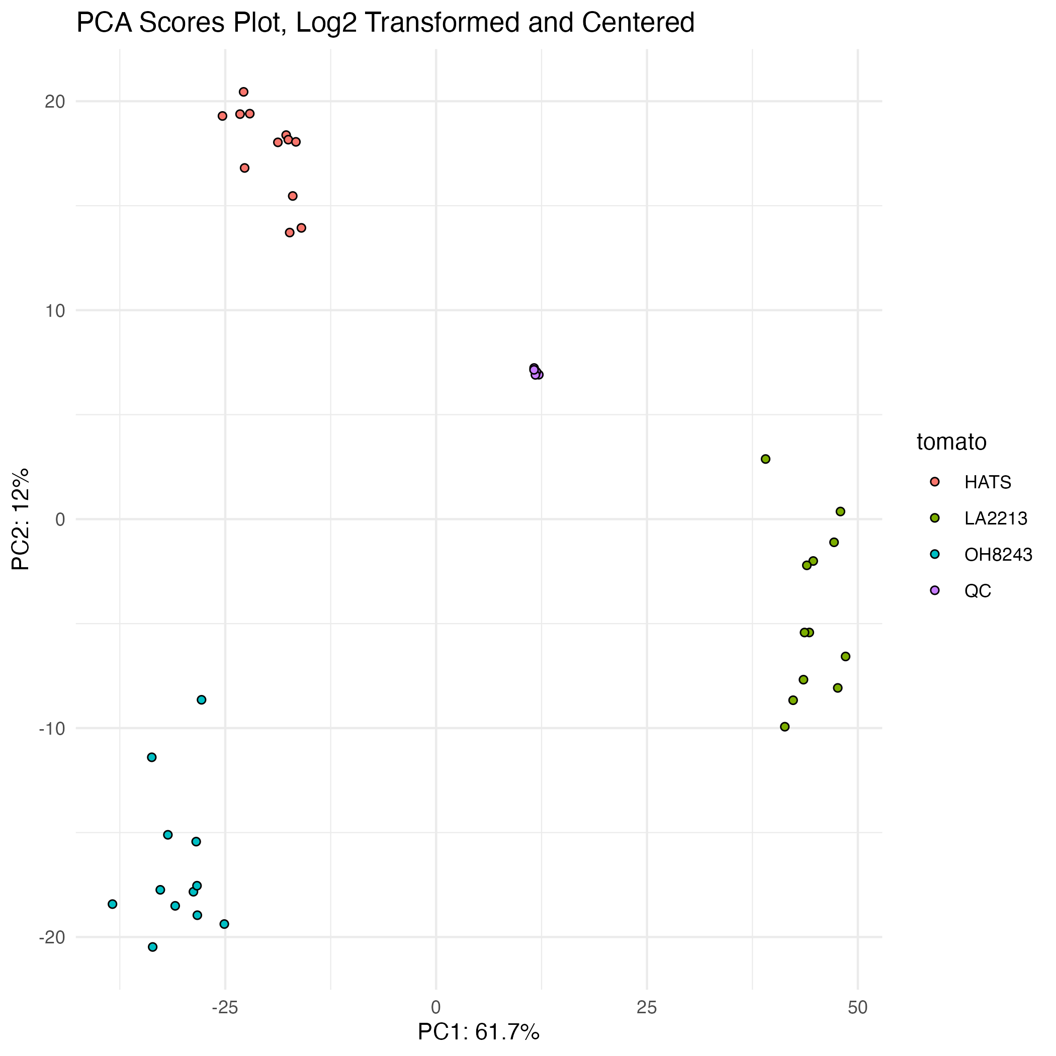
Centering

• Centering converts all relative intensities to be centered around zero instead of around mean concentrations
• This is particularly useful in metabolomics given that more intense features are not necessarily more abundant
• I like to center when conducting principal components analysis (PCA, more on this later)

PCA not centered

PCA centered

Scaling

• Uses data dispersion as a part of a scaling factor
  • Auto scaling: mean = 0, standard deviation = 1 (for each feature)
  • Pareto scaling: like auto but scaled to square root of the st dev. The most common scaling used for metabolomics
  • In general I find this not necessary and will just log transform (more coming next)

Log transformation - tables

• Reduce heteroscedasicity
• Makes large values proportionally smaller than small ones
• Makes distributions more normal

sample	feature_1	feature_2
control	10000	1000
treatment	11000	2000

sample	log2_feature_1	log2_feature_2
control	13.29	9.97
treatment	13.43	10.97

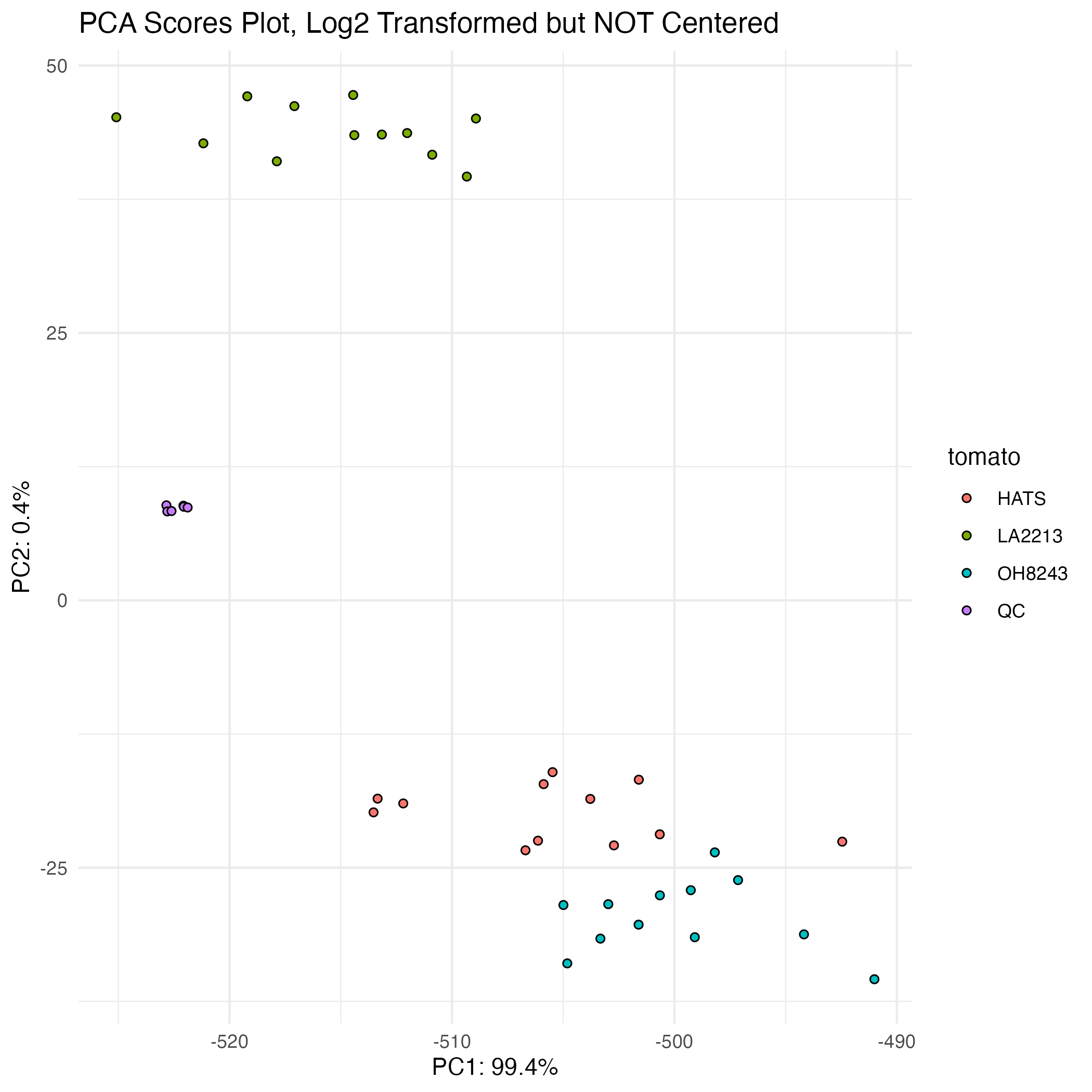
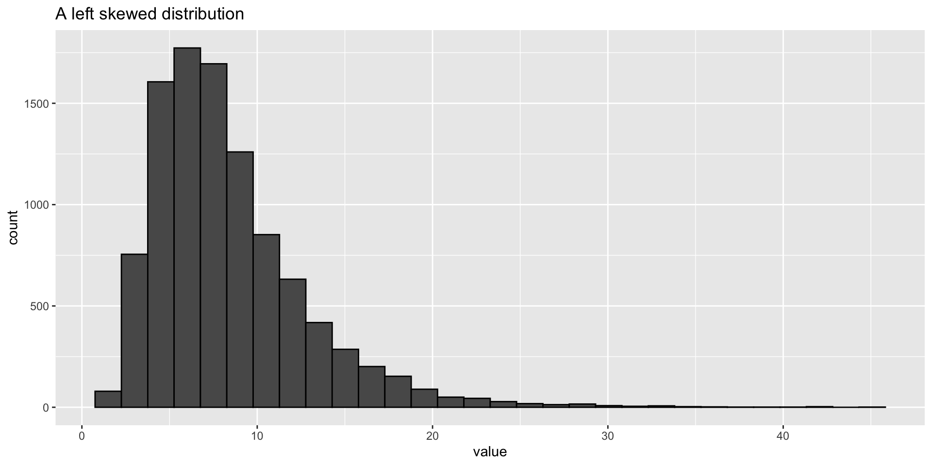
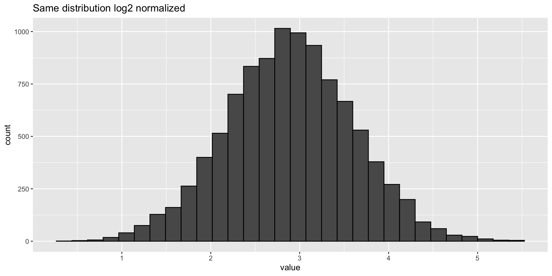
Log transformation - plots

• Log transforming can make your data look more normally distributed

Sample wise normalization

• Adjust based on weight or volume (very common)
• Adjust based on intensity of an internal standard (used sometimes)
• Adjust based on total signal (used in older MS papers and for NMR but not really in MS)

Assessing data quality

• How can we go about assessing if our data is of high quality when we have thousands of features and don’t know what to expect?

Overlay your BPCs

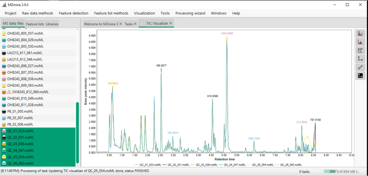
Overlaid base peak chromatograms in MZmine

Zoom in and look at your BPCs carefully

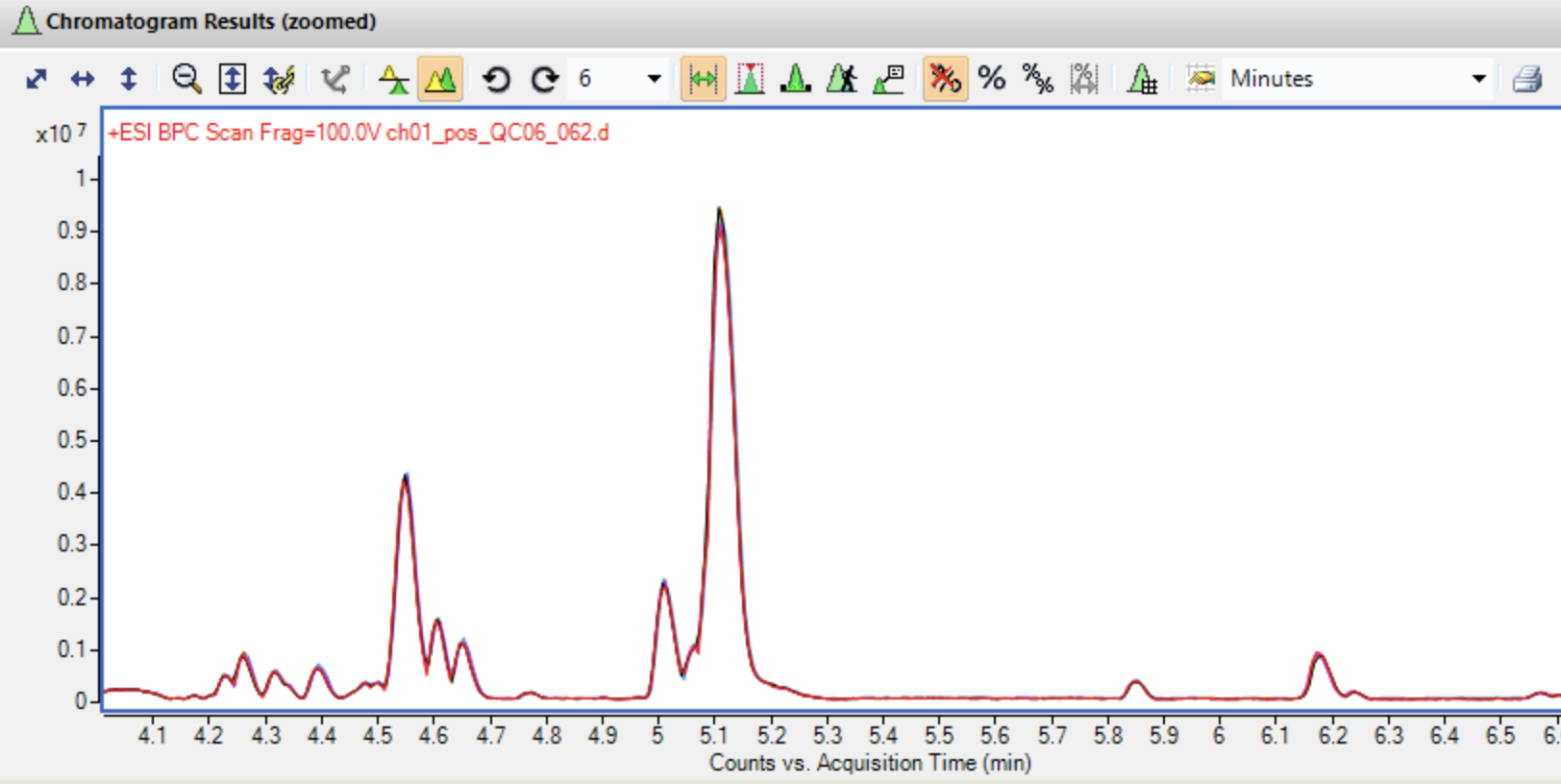
Overlaid base peak chromatograms in MassHunter

Look at a single feature for retention time shifting

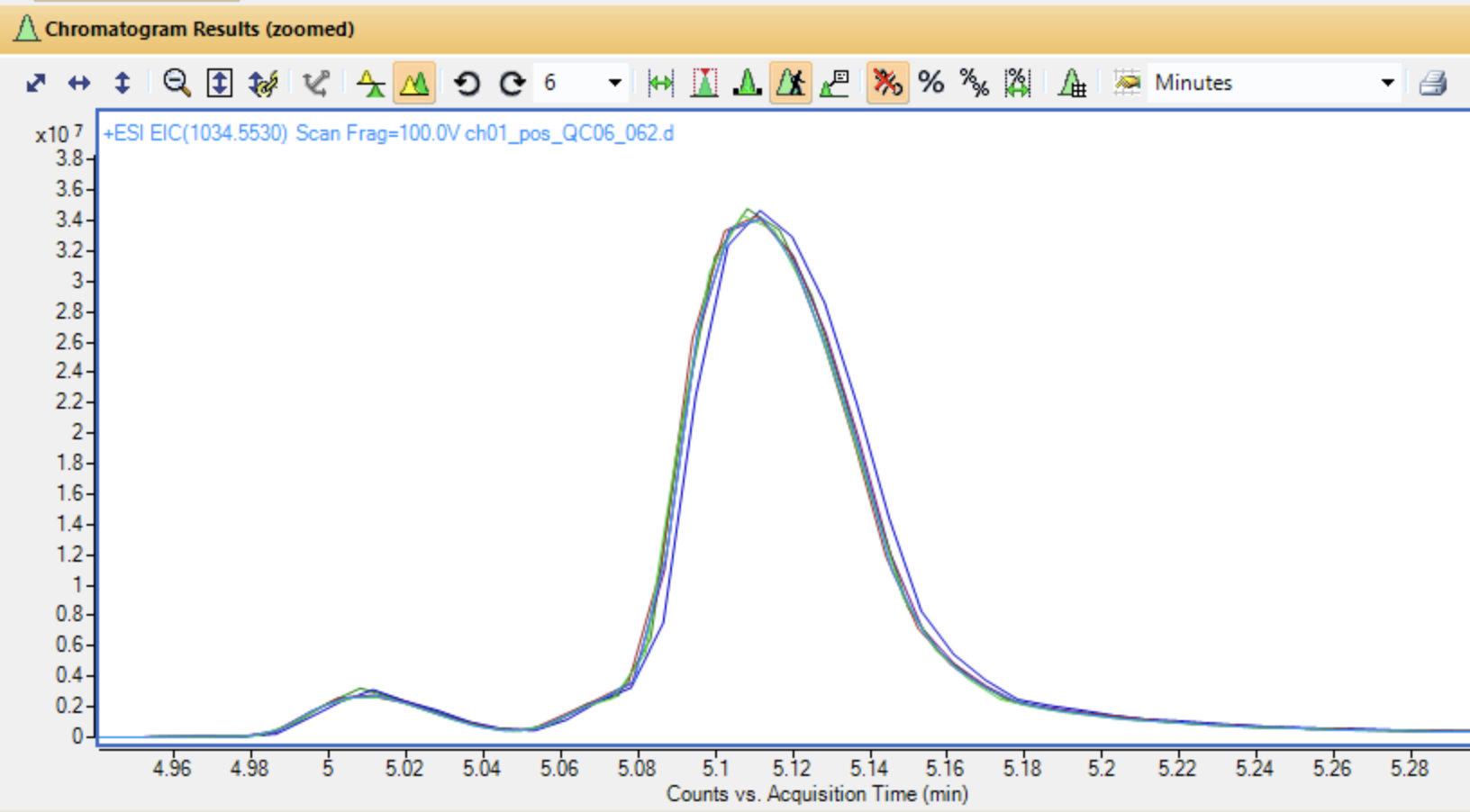
Overlaid extracted ion chromatograms in MassHunter

Create boxplots of features by sample

Ordering by sample groups

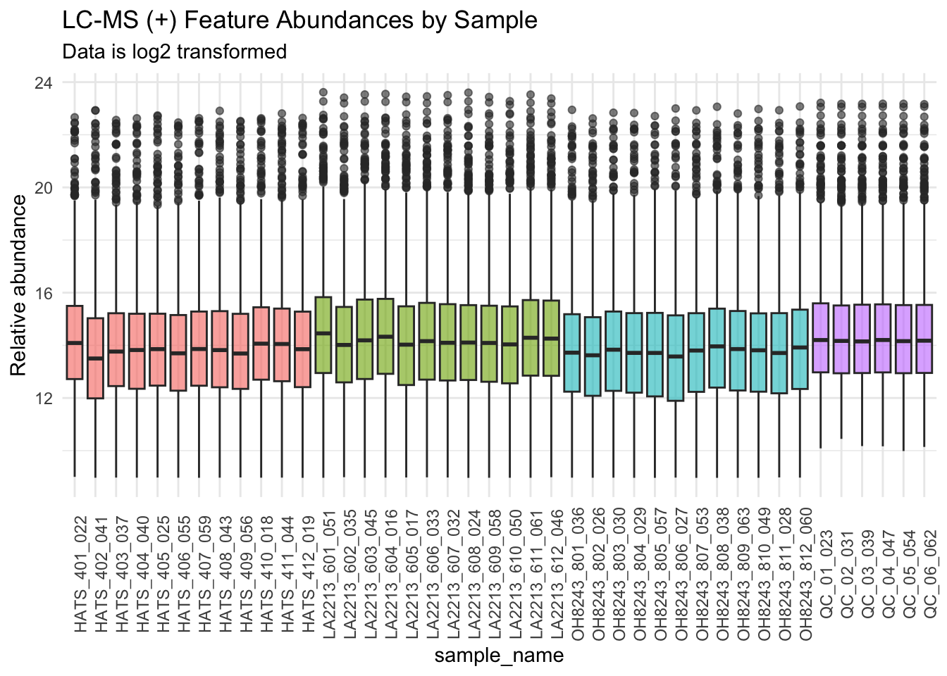
Ordering by run order

Your QCs should cluster in a PCA

A PCA where the QCs cluster beautifully

Data analysis can be unsupervised or supervised

Unsupervised (model does not know which samples belong to which groups):

• Principal components analysis (PCA)
• Hierarchical clustering analysis (HCA)
• K-means clustering

Supervised (model knows group composition):

• Univariate (or multivariate) group comparisons
• Predictive/classification models
  • Partial least squares regression (PLS-R)
  • PLS-discriminant analysis (PLS-DA)
  • Random forest
  • Artificial neural networks
  • Others

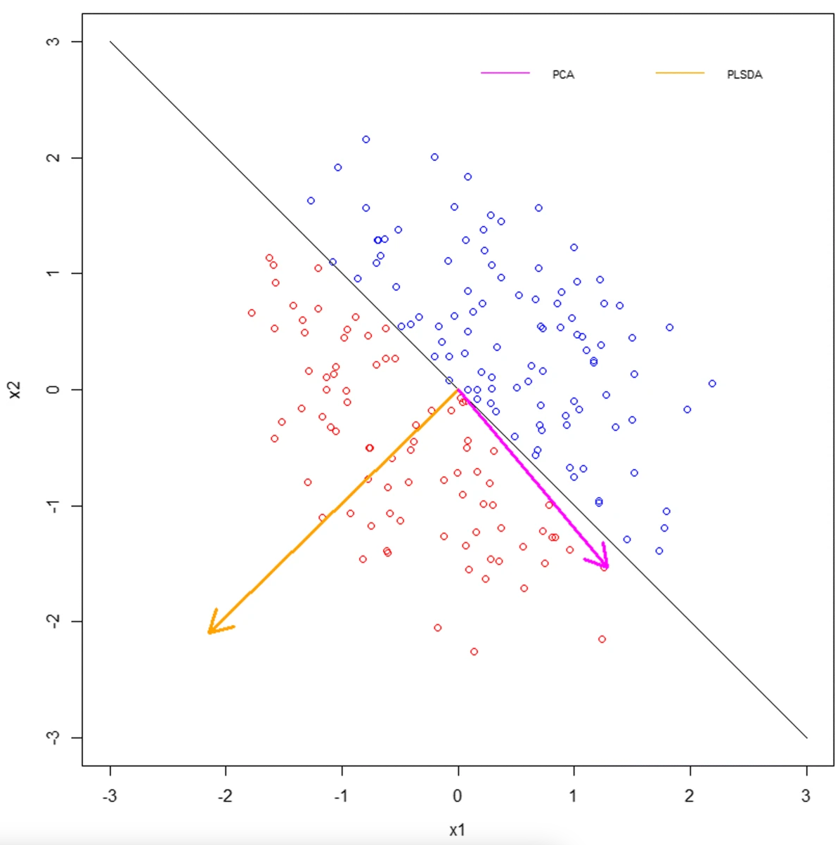
Unsupervised: Principal Components Analysis (PCA)

• A dimensionality reduction approach that transforms our data into a new system where principal coordinates (PCs) are drawn maximizing variation in our data.
• Each new PC is orthogonal to the previous one.
• Can interpret points closer together as more similar that those further apart
• The loadings plot helps us understand which features are most influential for each PC

Fig from https://www.ibm.com/topics/principal-component-analysis

Interpreting PCAs

PCA A) scores and B) loadings (from Dzakovich et al., 2022)

What you should be doing with your PCAs

• Check for samples that are very different from the rest
• Show that your QCs cluster together
• Look for batch effects
• Observe the distance between your samples within a group, and between groups
• See how much variation is being explained by each PC
• Look for clusters in your data

Unsupervised: Hierarchical Clustering Analysis (HCA)

• An approach to “cluster” samples based on their distance/similarity
• Find two most similar samples and merge into cluster, and repeat
• Different methods for determining both distance and linkage
• Like a phylogenic tree - samples that are closer together are more similar
• Can cluster samples, features, or both
• StatQuest video on hierarchical clustering

HCA applied to metabolomics

A hierarchical clustering example from Dzakovich et al., 2024

Unsupervised: K-means clustering

• Randomly assigns all samples to be a part of \(k\) clusters
• Calculates centroids and assigns samples to the nearest one
• Iterates until centroids stability or reach some maximum
• Can figure out number of clusters using a scree plot to visualize within cluster sums
• StatQuest explains K-means clustering

From Wikipedia

Supervised: Univariate testing, the categories

• Two group tests
  • t-test (parametric)
  • Wilcoxon rank sum test (non-parameric)
• More than two group tests
  • ANOVA (parametric)
  • Kruskal Wallis test (non-parametric)
  • Both followed by post-hoc means separation

Big p, little n: the curse of high dimensionality

• With metabolomics, we almost always have more features (p) than samples (n)
• This means we are making a lot of comparisons
• If we want to know if each feature is differentially abundant across two groups, we can do a series of t-tests.
• If we set α = 0.05, then we have a 5% chance for rejecting the null when it is true (false positive, type I error)
• If we do 1000 tests, and each one has a 5% of a false positive, then we would predict to have 50 false positives due to chance alone - features that have p < 0.05 but are not truly different between our groups

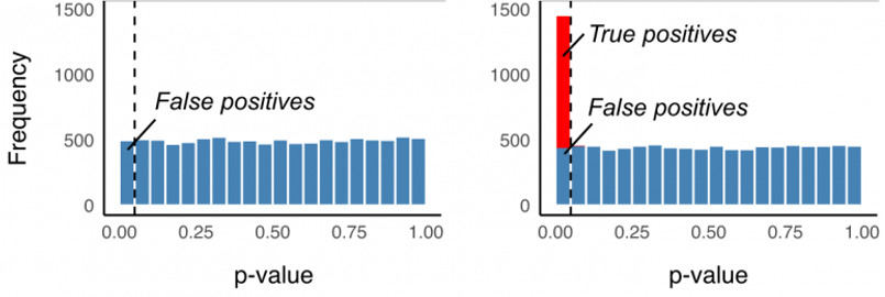
Ways to control for multiple testing

• Bonferroni correction: \(α/number\,of\,comparisons\) (very conservative, leads to false negatives)
• Benjamini Hochberg false discovery rate correction: adjust overall error rate to be α (tries to balance false negatives and positives)

Fig. from https://geneviatechnologies.com/blog/what-is-multiple-testing-correction/

Should I use parametric or non-parametric tests?

Multivariate testing in metabolomics

• Multivariate approaches allow the investigation of more than one feature at once
• Approaches can be unsupervised or supervised
• Be sure to select the most appropriate method given the nature of your data and question

Supervised: PLS-DA

• Partial least squares discriminate analysis (PLS-DA) approaches optimize separation between groups
• Two data matrices, X: contains your features, Y: contains group identity
• Be sure to look at R^2 and Q^2 for both training and test sets
• Has a tendency to overfit
• Learn more about PLS-DA: Brereton and Lloyd, J Chemometrics 2014, Ruiz-Perez et al., BMC Bioinformatics 2020, Worley and Powers, Curr Metabolomics 2013.

Ruiz-Perez et al., BMC Bioinformatics 2020

Random forest

• A machine learning method for classification via construction of decision trees
• Trees are created with a random subset of variables
• Increase to 100% purity at the base of the tree
• Do this over and over
• A set (~1/3rd) is left out of the sample for each tree - this is the “out of bag (oob)” data, and can be used to see how accurate your classification is
• Learn more by watching this StatQuest video

An example of a simple, single decision tree

Artificial neural networks

• Conceptually like a network of connected neurons, where each connection is weighted and a function transforms the sums to form the output
• Input data is mapped to latent structures, which are then mapped to output data
• Sometimes can be a “black box”
• Learn more by watching this StatQuest video

An illustration of a single neural network, from Mendez et al., Metabolomics 2019

Others